Power

note

Power analysis is currently in alpha (version 2.9+ required). To enable power analysis, go to your organizational settings, and toggle "Enable Power Calculator" in "Experiment Settings." Currently GrowthBook offers only frequentist power analysis. Bayesian power analysis is coming soon.

What is power analysis?

Power analysis helps you estimate required experimental duration. Power is the probability of observing a statistically significant result, given your feature has some effect on your metric.

When should I run power analysis?

You should run power analysis before your experiment starts, to determine how long you should run your experiment. The longer the experiment runs, the more users are in the experiment (i.e., your sample size increases). Increasing your sample size lowers the uncertainty around your estimate, which makes it likelier you achieve a statistically significant result.

What is a minimum detectable effect, and how do I interpret it?

Recall that your relative effect size (which we often refer to as simply the effect size), is the percentage improvement in your metric caused by your feature. For example, suppose that average revenue per customer under control is $100, while under treatment you expect that it will be $102. This corresponds to a ($102-$100)/$100 = 2% effect size. Effect size is often referred to as lift.

Given the sample variance of your metric and the sample size, the minimum detectable effect (MDE) is the smallest effect size for which your power will be at least 80%.

GrowthBook includes both power and MDE results to ensure that customers comfortable with either tool can use them to make decisions. The MDE can be thought of as the smallest effect that you will be able to detect most of the time in your experiment. We want to be able to detect subtle changes in metrics, so smaller MDEs are better.

For example, suppose your MDE is 2%. If you feel like your feature could drive a 2% improvement, then your experiment is high-powered. If you feel like your feature will probably only drive something like .5% improvement (which can still be huge!), then you need to add users to detect this effect.

How do I run a power analysis?

1. From the GrowthBook home page, click "Experiments" on the left tab. In the top right, click "+ Power Calculation."
2. Select “New Calculation”.
3. On the first page you:

• Select your metrics (maximum of 5). Currently binomial, count, duration, and revenue metrics are supported, while ratio and quantile metrics are unsupported.
• Select your "Estimated users per week." This is the average number of new users your experiment will add each week. See FAQ below for a couple of simple estimation approaches.
• click "Next".

4. On the second page you:

• enter the "Effect Size" for each metric. Effect size is the percentage improvement in your metric (i.e., the lift) you anticipate your feature will cause. Inputting your effect size can require care - see here.
• for binomial metrics, enter the conversion rate.
• for other metrics, enter the metric mean and metric standard deviation. These means and standard deviations occur across users in your experimental population.
• click "Next".

5. Now you have results! Please see the results interpretation here.
6. By clicking "Edit" in the "Analysis Settings" box, you can toggle sequential testing on and off to compare power. Enabling sequential testing decreases power.
7. You can alter the number of variations in your experiment. Increased variations result in smaller sample sizes per variation, resulting in lower power.
8. If you want to modify your inputs, click the "Edit" button next to "New Calculation" in the top right corner.

How do I interpret power analysis results?

In this section we run through an example power analysis. After starting power analysis, you will need to select metrics and enter estimated users per week.

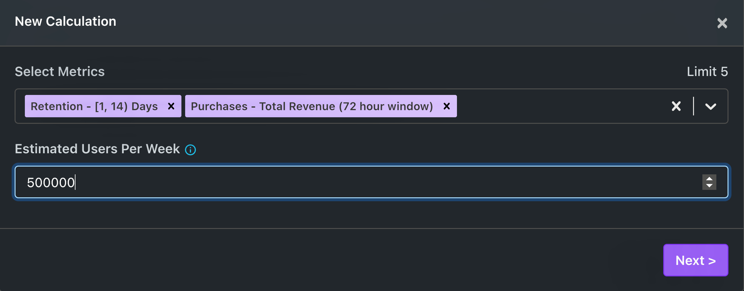
In our example, we choose a binomial metric (Retention - [1, 14) Days) and a revenue metric (Purchases - Total Revenue (72 hour window)). We refer to these metrics as "retention" and "revenue" respectively going forward. We estimate that 500,000 new users per week visit our website.

You then input your effect sizes, which are the best guesses for your expected metric improvements due to your feature.

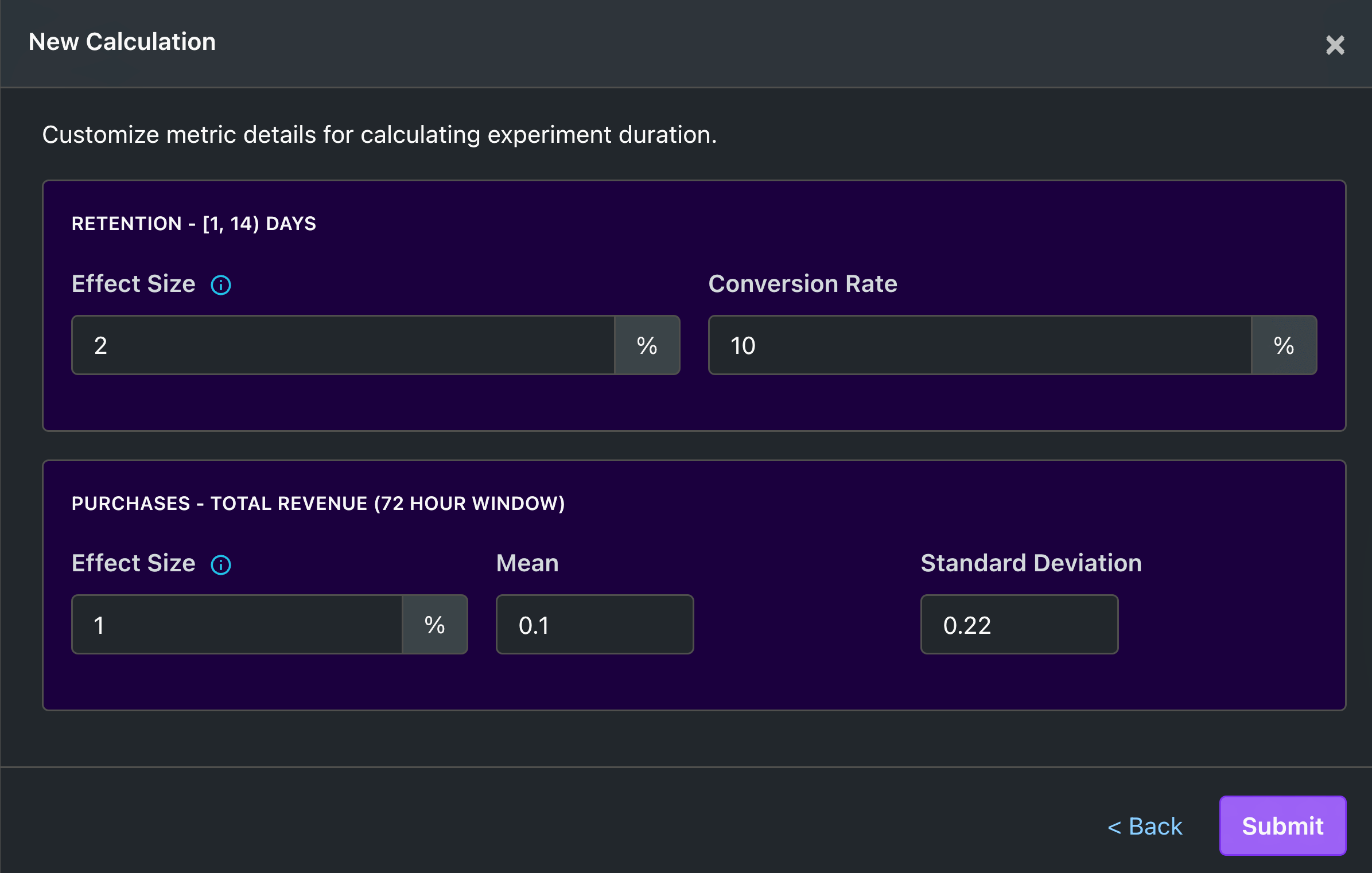
We provide guidance for effect size selection here. For our feature we anticpate a 2% improvement in retention. For retention, the conversion rate is 10%. This 10% number should come from an offline query that measures your conversion rate on your experimental population. We expect a 1% improvement in revenue, which has a mean of $0.10 and a standard deviation of $0.22 (as with conversion rate, the mean and standard deviation come from an offline query that you run on your population). We then submit our data.

Now we can see the results!

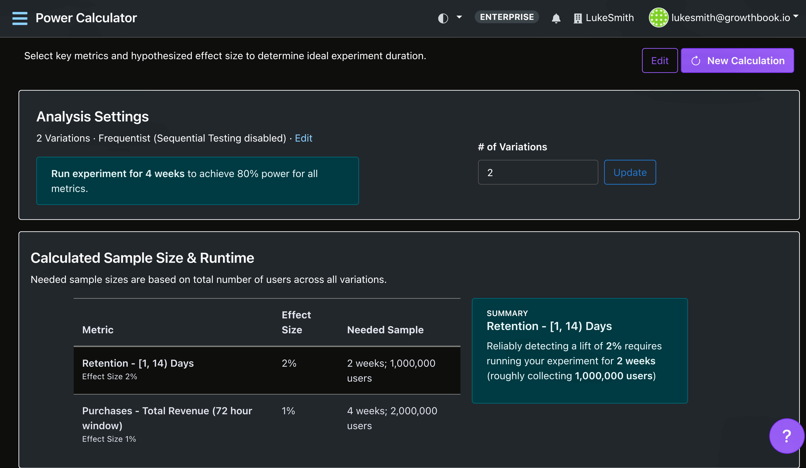
At the top of the page is a box called Analysis Settings. The summary here says, "Run experiment for 4 weeks to achieve 80% power for all metrics." This is the most important piece of information from power analysis. If running your experiment for 4 weeks is compatible with your business constraints, costs, and rollout timeframe, then you do not need to dive into the numbers below this statement. If you want to rerun power results with number of variations greater than 2, then click "# of Variations" and then click "Update". If you want to toggle on or off "Sequential Testing", then press the "Edit" button and select the appropriate option. Enabling sequential testing reduces power.

Below "Analysis Settings" is "Calculated Sample Size and Runtime", which contains the number of weeks (or equivalently the number of users) needed to run your experiment to achieve 80% power by metric. Clicking on a row in the table causes the information in the box to the right to change. We expect 80% power for retention if we run the experiment for 2 weeks. For revenue, we need to run the experiment for 4 weeks to achieve at least 80% power.

Beneath "Calculated Sample Size and Runtime" is "Power Over Time", which contains power estimates by metric.

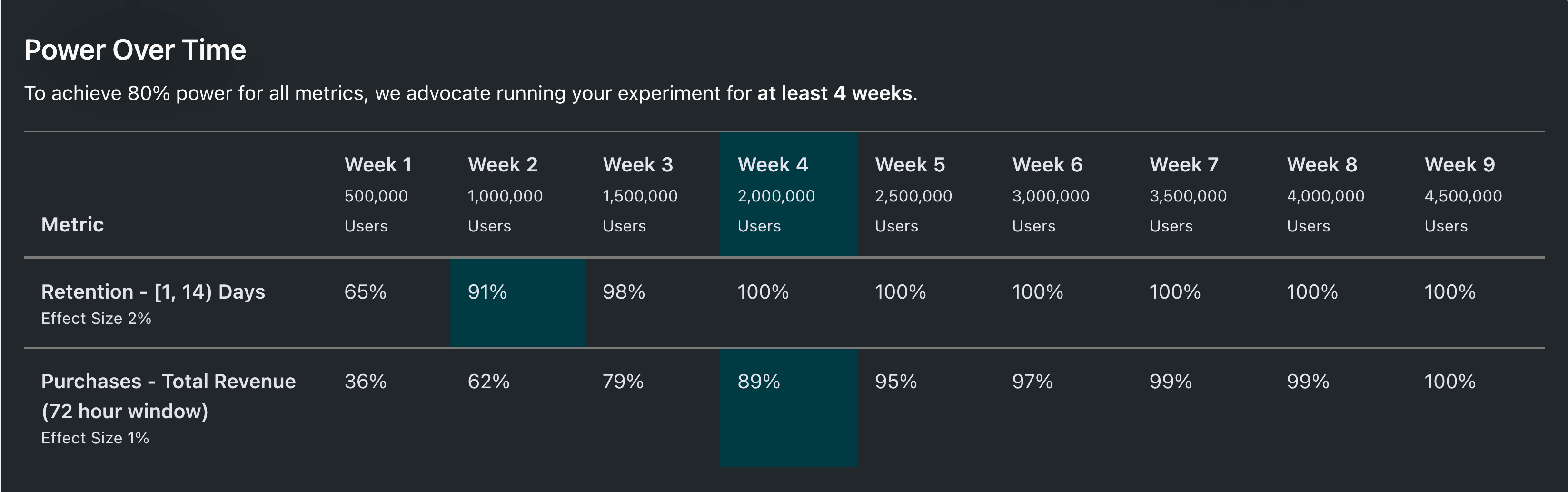
The columns in Power Over Time correspond to different weeks. For example, in the first week power for retention is 65%. The highlighted column in week 4 is the first week where at least 80% power is achieved for all metrics. As expected, power increases over time, as new users are added to the experiment.

Beneath Power Over Time is Minimum Detectable Effect Over Time.

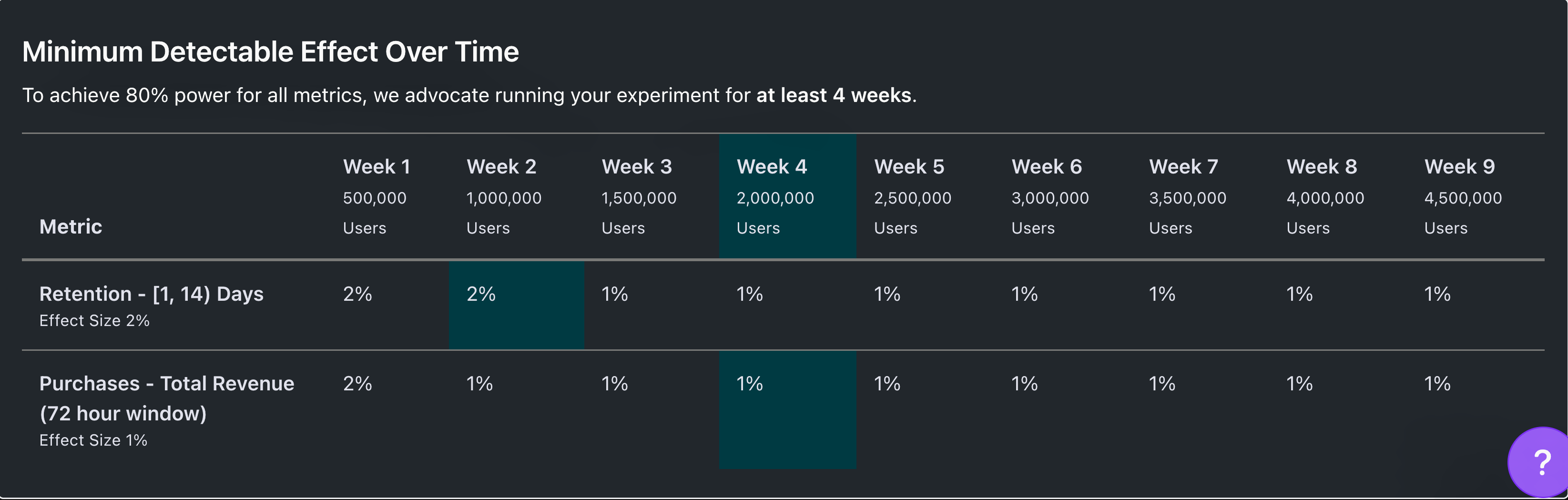
Minimum Detectable Effect Over Time is structured the same as Power Over Time, except it contains MDEs rather than power estimates. The Week 1 revenue MDE is 2%. This means that if your true lift is 2%, after 1 week you will have at least 80% chance of observing a statistically significant result. As expected, MDEs decrease over time, as new users are added to the experiment.

If you see N/A in your MDE results, this means that you need to increase your number of weekly users, as the MDE calculation failed.

It can be helpful to see power estimates at different effect sizes, different estimates of weekly users, etc. To modify your inputs, click the "Edit" button next to "New Calculation" in the top right corner.

How should I pick my effect size?

Selecting your effect size for power analysis requires careful thought. Your effect size is your anticipated metric lift due to your feature. Obviously you do not have complete information about the true lift, otherwise you would not be running the experiment!

We advocate running power analysis for multiple effect sizes. The following questions may elicit helpful effect sizes:

1. What is your best guess for the potential improvement due to your feature? Are there similar historical experiments, or pilot studies, and if so, what were their lifts?
2. Suppose your feature is amazing - what do you think the lift would be?
3. Suppose your feature impact is smaller than you think - how small could it be?

Ideally your experiment has high power (see here) across a range of effect sizes.

What is a high-powered experiment?

In clinical trials, the standard is 80%. This means that if you were to run your clinical trial 100 times with different patients and different randomizations each time, then you would observe statistically significant results in at least roughly 80 of those trials. When calculating MDEs, we use this default of 80%.

That being said, running an experiment with less than 80% power can still help your business. The purpose of an experiment is to learn about your business, not simply to roll out features that achieve statistically significant improvement. The biggest cost to running low-powered experiments is that your results will be noisy. This usually leads to ambiguity in the rollout decision.

FAQ

Frequently asked questions:

1. How do I pick the number for Estimated Users Per Week? If you know your number of daily users, you can multiply that by 7. If traffic varies by day of the week, you may want to do something like (5 average weekday traffic + 2 average weekend traffic) / 7.
2. How can I increase my experimental power? You can increase experimental power by increasing the number of daily users, perhaps by either expanding your population to new segments, or by including a larger percentage of user traffic in your experiment. Similarly, if you have more than 2 variations, reducing the number of variations increases power.
3. What if my experiment is low-powered? Should I still run it? The biggest cost to running a low-powered experiment is that your results will probably be noisy, and you will face ambiguity in your rollout/rollback decision. That being said, you will probably still have learnings from your experiment.
4. What does "N/A" mean for my MDE result? It means there is no solution for the MDE, given the current number of weekly users, control mean, and control variance. Increase your number of weekly users or reduce your number of treatment variations.

GrowthBook implementation

Below we describe technical details of our implementation. First we start with the definition of power.
Define:

1. the false positive rate as $\alpha$ (GrowthBook default is $\alpha=0.05$).
2. the critical values $Z_{1-\alpha/2}= \Phi^{-1}(1-\alpha/2)$ and $Z_{1-\alpha}= \Phi^{-1}(1-\alpha)$ where $\Phi$ is the inverse CDF of the standard normal distribution.
3. the true relative treatment effect as $\tau$, its estimate as $\hat{\tau}$ and its estimated standard error as $s$. Note that as the sample size $n$ increases, s decreases by a factor of $1/\sqrt{n}$.

We make the following assumptions:

1. equal sample sizes across control and treatment variations;
2. equal variance across control and treatment variations;
3. observations across users are independent and identically distributed; and
4. all metrics have finite variance.
5. you are running a two-sample t-test. If in practice you use CUPED, your power will be higher. Use CUPED!

For a 1-sided test, the probability of a statistically significant result (i.e., the power) is

$\pi = P\left(\frac{\hat{\tau}}{s} > Z_{1-\alpha}\right)=P\left(\frac{\hat{\tau}-\tau}{s} > Z_{1-\alpha}-\frac{\tau}{s}\right)=1 - \Phi\left(Z_{1-\alpha}-\frac{\tau}{s}\right)$.

For a 2-sided test (all GrowthBook tests are 2-sided), the power is composed of the probability of a statistically significant positive result and a statistically significant negative result. Using the same algebra as above (except using $Z_{1-0.5\alpha}$ for the critical value), the probability of a statistically significant positive result is $\pi_{pos} = 1 - \Phi\left(Z_{1-\alpha/2}-\frac{\tau}{s}\right)$. The probability of a statistically significant negative result is $\pi_{neg} = P\left(\frac{\hat{\tau}}{s} < Z_{\alpha/2}\right)=P\left(\frac{\hat{\tau}-\tau}{s} < Z_{\alpha/2}-\frac{\tau}{s}\right)=\Phi\left(Z_{\alpha/2}-\frac{\tau}{s}\right)$.
For a 2-sided test, the power equals

$\pi = 1 - \Phi\left(Z_{1-\alpha/2}-\frac{\tau}{s}\right) + \Phi(Z_{\alpha/2} - \frac{\tau}{s})$.

The MDE is the smallest $\tau$ for which nominal power (i.e., 80%) is achieved. For a 1-sided test there is a closed form solution for the MDE. Solving the 1-sided power equation for $\tau$ produces $\text{MDE} = s\left(Z_{1-\alpha/2}-\Phi^{-1}(1 - \pi)\right) = s\left(\Phi^{-1}(1 - \alpha/2)-\Phi^{-1}(1 - \pi)\right)$.

In the 2-sided case there is no closed form solution, so we instead invert the equation below, which ignores the neglible term $\Phi(Z_{\alpha/2} - \frac{\tau}{s})$, and produces power estimates very close to 0.8:

$\pi = 1 - \Phi\left(Z_{1-\alpha/2}-\frac{\tau}{s}\right)$

One subtlety with finding MDEs for relative treatment effects is that the uncertainty of the estimate depends upon the mean. So when inverting the power formula above to find the minimum $\tau$ that produces at least 80% power, the uncertainty term $s$ changes as $\tau$ changes.
We solve for the equation below, where we make explicit the dependence of $s$ on $\tau$:

$\frac{\tau}{s(\tau)} = \Phi^{-1}\left({1-\alpha/2}\right) - \Phi^{-1}(1 - \pi).$

Define $\mu_{A}$ as the population mean of variation $A$ and $\sigma^{2}$ as the population variance. For variation $B$ analogously define $\mu_{B}$; recall that we assume equal variance across treatment arms.
Define $N$ as the per-variation sample size. Define the sample counterparts as ($\hat{\mu}_{A}$, $\hat{\sigma}_{A}^{2}$, $\hat{\mu}_{B}$, and $\hat{\sigma}_{B}^{2}$).

Recall that our lift is defined as $\tau = (\mu_{B}-\mu_{A})/\mu_{A}$ and the variance of the sample lift $\hat{\tau} = (\hat{\mu_{B}}-\hat{\mu_{A}})/\hat{\mu_{A}}$ is

$\text{Var}(\hat{\tau}) = \frac{\sigma^{2}}{N}\frac{1}{\mu_{A}^{2}} + \frac{\sigma^{2}}{N} *\frac{\mu_{B}^{2}}{\mu_{A}^{4}}.$

Define the constant $k = \Phi^{-1}\left({1-\alpha/2}\right) - \Phi^{-1}(1 - \pi)$. We solve for $\mu_{B}$ in:

$\frac{(\mu_{B}-\mu_{A})/\mu_{A}}{\sqrt{\text{Var}(\hat{\tau})}} = k^{2} \iff (\mu_{B}-\mu_{A})^{2} =k^{2}\mu_{A}^{2}\text{Var}(\hat{\tau}) = k^{2}\mu_{A}^{2}\left(\frac{\sigma^{2}}{N}\frac{1}{\mu_{A}^{2}} + \frac{\sigma^{2}}{N} *\frac{\mu_{B}^{2}}{\mu_{A}^{4}}\right).$

Rearranging terms shows that $\mu_{B}^{2}\left(1-\frac{\sigma^{2}}{N}\frac{k^{2}}{\mu_{A}^{2}}\right) + \mu_{B}\left(-2\mu_{A}\right) + \left(\mu_{A}^{2}-k^{2}\frac{\sigma^{2}}{N}\right) = 0.$

This is quadratic in $\mu_{B}$ and has solution

$$\mu_{B} = \frac{2 \mu_{A} \pm \sqrt{4 \mu_{A}^{2}-4\left(1-\frac{\sigma^{2}}{N}\frac{k^{2}}{\mu_{A}^{2}}\right)\left(\mu_{A}^{2}-k^{2}\frac{\sigma^{2}}{N}\right)}}{2\left(1-\frac{\sigma^{2}}{N}\frac{k^{2}}{\mu_{A}^{2}}\right)} = \frac{\mu_{A} \pm \sqrt{\mu_{A}^{2}-\left(1-\frac{\sigma^{2}}{N}\frac{k^{2}}{\mu_{A}^{2}}\right)\left(\mu_{A}^{2}-k^{2}\frac{\sigma^{2}}{N}\right)}}{\left(1-\frac{\sigma^{2}}{N}\frac{k^{2}}{\mu_{A}^{2}}\right)} .$$

The discriminant reduces to

$k^{2} * \frac{\sigma^{2}}{N} \left(2 - \frac{\sigma^{2}}{N} * \frac{k^{2}}{\mu_{A}^{2}}\right).$

so a solution for $\mu_{B}$ exists if and only if

$$2 - \frac{\sigma^{2}}{N} * \frac{k^{2}}{\mu_{A}^{2}} > 0 \iff 2 > \frac{\sigma^{2}}{N} * \frac{k^{2}}{\mu_{A}^{2}} \iff N > \frac{\sigma^{2}k^{2}}{2\mu_{A}^{2}}.$$

Similarly, the MDE returned can be negative if the denominator is negative, which is nonsensical.
We return cases only where the denominator is positive, which occurs if and only if:

$\left(1-\frac{\sigma^{2}}{N}\frac{k^{2}}{\mu_{A}^{2}}\right) > 0 \iff \left(1-\frac{\sigma^{2}}{N}\frac{k^{2}}{\mu_{A}^{2}}\right) > 0 \iff N > \frac{\sigma^{2}k^{2}}{\mu_{A}^{2}}.$

This condition is stricter than the condition guaranteeing existence of a solution.

Therefore, there will be some combinations of $(\mu_{A}, \sigma_{2})$ where the MDE does not exist for a given $N$. If $\alpha=0.05$ and $\pi=0.8$, then $k\approx 2.8$. Therefore, a rule of thumb is that $N$ needs to be roughly 9 times larger than the ratio of the variance to the squared mean to return an MDE. In these cases, $N$ needs to be increased.

To estimate power under sequential testing, we adjust the variance term $s$ to account for sequential testing, and then input this adjusted variance into our power formula. We assume that you look at the data only once, so our power estimate below is a lower bound for the actual power under sequential testing. Otherwise we would have to make assumptions about the temporal correlation of the data generating process.

In sequential testing we construct confidence intervals as

$\left(\hat{\tau} \pm \hat{\sigma}*\sqrt{N} * \sqrt{\frac{2(N\rho^2 + 1)}{N^2\rho^2}\log\left(\frac{\sqrt{N\rho^2 + 1}}{\alpha}\right)}\right)$

where

$\rho = \sqrt{\frac{-2\text{log}(\alpha) + \text{log}(-2 \text{log}(\alpha) + 1)}{N^*}}$

and $N^{\star}$ is a tuning parameter. This approach relies upon asymptotic normality. For power analysis we rewrite the confidence interval as

$\left(\hat{\tau} \pm \hat{\sigma}*\sqrt{N} * \sqrt{\frac{2(N\rho^2 + 1)}{N^2\rho^2}\log\left(\frac{\sqrt{N\rho^2 + 1}}{\alpha}\right)}\frac{Z_{1-\alpha/2}}{Z_{1-\alpha/2}}\right)$$=\left(\hat{\tau} \pm \tilde{\sigma}Z_{1-\alpha/2}\right)$

where

$\tilde{\sigma} = \hat{\sigma}*\sqrt{N}\sqrt{\frac{2(N\rho^2 + 1)}{N^2\rho^2}\log\left(\frac{\sqrt{N\rho^2 + 1}}{\alpha}\right)}\frac{1}{Z_{1-\alpha/2}}$.

We use power analysis described above, except we substitute $\tilde{\sigma}^{2}$ for $s^{2}$.